In our forecast discussion, we will occasionally mention things like “limited dispersion” or “low mixing heights” – have you ever wondered what that means? It means that we are expecting limited dispersion of air pollution, or to put it another way–if there’s some air pollution around it won’t be going very far! Dispersion of air pollution occurs in both the vertical and horizontal direction.
Horizontal Dispersion
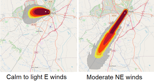
Horizontal dispersion is how far and wide pollution spreads at a given level of the atmosphere (we focus on ground-level pollution here at the NCDAQ). It is primarily driven by wind speed and direction, but can be influenced by topography as well. Where air pollution ends up—be it a locally generated plume of ozone or smoke from a large wildfire—will largely depend on where the wind is blowing from, and how fast it’s blowing. For example, consider a small controlled burn that emits smoke particles for a couple of hours. The image below was created using a dispersion model called HYSPLIT, and simulates the dispersion of a hypothetical controlled burn with real meteorological data to demonstrate how wind speed and direction can affect dispersion. On a day with light easterly winds (i.e. winds blowing from the east), areas to the west immediately near and downwind (direction the wind is blowing to) of the fire will see the highest concentrations of smoke, with decreasing concentrations further out. As the plume of smoke is blown by the wind, it will spread not only westward, but drift outwards from its centerline (an imaginary line drawn down the center of the plume as viewed from above) to the north and south as it moves to the west. Now consider the same controlled burn on a day with moderate northeasterly speeds–the highest concentrations will still be in the middle of the plume, though faster wind speeds will not allow it to spread as far outwards from the centerline, resulting in a more elongated plume that reaches a further distance away. Note that horizontal dispersion can be affected by topography—for example, sometimes pollution will be blown into the entrance of a valley where it can remain trapped if the wind speeds aren’t enough to carry it over the ridges that define it. This happens on a larger scale in a city like Los Angeles that is surrounded by mountains on three sides.
Vertical Dispersion
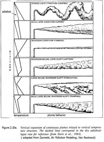
For dispersion in the vertical, it’s all about thermodynamics! Have you ever heard the phrase “warm air rises?” This is something to keep in mind when thinking about vertical dispersion. When air quality forecasters prepare forecasts, one thing that is analyzed is the vertical temperature and wind profile of the atmosphere, also known as an “atmospheric sounding.” This data is either obtained from forecast models or via real-world measurements from weather balloons. Consider this: imagine taking an imaginary box full of air at the surface, also known as a “parcel of air.” As the morning sun heats the surface the parcel of air will rise. Typically, the atmosphere cools with height, so as the parcel of air ascends it will be warmer than the air surrounding it and keep rising. However, sometimes the air near the surface (often at night) will cool below the temperature of the air above it, resulting in temperatures that increase with height – this is known as a surface temperature inversion. If one were to lift a parcel of air from the surface upwards during a temperature inversion, that parcel of air will be cooler than the air surrounding it and sink back to the surface. Now imagine that parcel of air representing air pollution – it is effectively trapped near the surface during a surface temperature inversion, and is not able to readily disperse vertically. The top of the inversion helps to indicate the “mixing height,” which is essentially the level below which the air will readily mix. Thankfully, as the lower atmosphere continues to be warmed by the sun, an overnight temperature inversion will erode and mixing heights increase and allow for better mixing of the air. You may have noticed this phenomenon if you are ever outside in the early morning of January 1st or July 5th following New Years Eve/July 4th firework displays – sometimes the air seems hazy/smokey, and it’s usually thanks in part to a low-level temperature inversion trapping the celebratory smoke. The image below features a diagram of six different atmospheric temperature profiles, and demonstrates how pollution can disperse in the vertical based on the temperature profile of the atmosphere (height on the Y-axis, temperature on the X-axis).
Atmospheric Profiles
The image below shows two different forecast atmospheric soundings. The right side of each sounding shows how the wind speed and direction change with height. The wind barbs point to where the wind is coming from, and the longer the barb on the end, the swifter the winds. Which do you think will offer better dispersion?
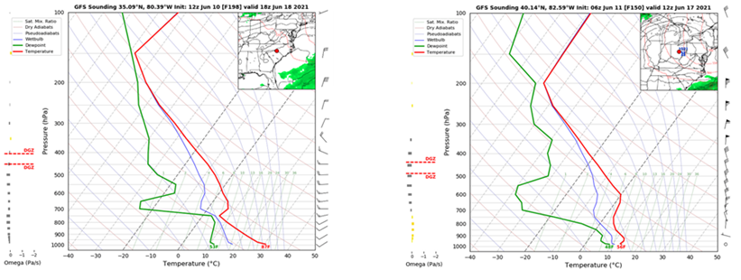
The sounding on the left shows an atmosphere readily cooling with height, and moderate winds from the surface to the upper atmosphere (albeit with an inversion around 750mb). The sounding on the right shows a small low-level inversion, with calm to light winds up to the 700mb height. If you guessed the one on the left, you are correct! The swifter wind speeds will help to mix the air and reduce pollution concentrations by enhancing horizontal dispersion at all levels through the atmosphere.
Long-Range Transport
When there is a large source of air pollution, or if it lofts high above the surface, upper-level winds can help to transport it large distances—sometimes even spanning the continent!
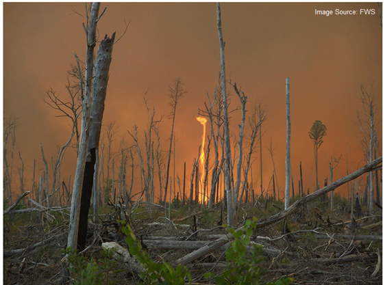
Wildfire season out in the western states can have huge impacts locally, but when fires burn for days and weeks then massive amounts heat and smoke are produced. As mentioned above, “warm air rises,” and the massive amounts of heat aid to lift the smoke far up and away from the surface. This is also why there will occasionally be a “fire tornado” or “fire whirl” in large fires—upwards air currents lift the burning flames, resulting in a fire whirl, which is a good way to visualize the phenomenon of warm air rising.
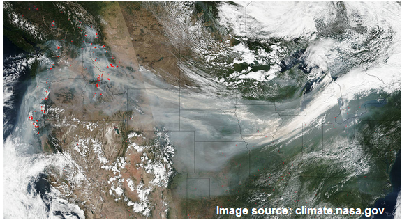
As the massive amounts of smoke reach the mid-upper levels of the atmosphere, upper-level winds (and the jet stream) can carry the smoke long distances, spanning countries or even continents!
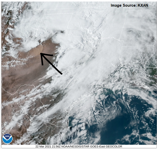
In addition to smoke, dust can reach long distances as well. Here in the United States, West Texas is home to the Permian Basin and parts of the Chihuahuan Desert. When the land is dry and winds are strong enough (often as a strong, dry cold front advances), large amounts of blowing dust can be generated, and the finer the dust, the longer it will take to settle out of the air mass. In far West Texas, the city of El Paso sits to the east/northeast of a dried up lakebed (Lake Palomas), which contains very fine dust. Since the dust is so fine it is easily disturbed by winds and in this region blowing dust events can happen a couple times a year. Blowing dust often pools along a frontal boundary as it advances, occasionally bringing elevated levels of fine particle pollution all the way across the state! This type of event happens in other desert locations as well, such as Arizona and New Mexico. In areas near and immediately downwind of the source region of the dust, it’s not uncommon for daily fine particle pollution AQIs to reach Code Red, or even Code Purple levels.
Super Long-Range Transport
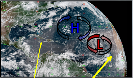
Believe it or not, dust from the Saharan Desert in Africa can (and does with some regularity) traverse across the entire Atlantic Ocean! The Saharan Desert region was once under water, and the sand is very fine and rich in nutrients and minerals from ancient decomposed marine life. Strong winds in the summertime generate massive amounts of blowing dust, far beyond what’s generated here in the desert regions of the United States. Prevailing easterly winds carry the dust across the ocean, reaching North and South America. The dust is beneficial in that it provides nutrients to the Amazon Rain Forest but can cause elevated levels of fine particle pollution in the southeastern United States. Florida and states along the Gulf Coast region are more likely to see high concentrations of dust, but on occasion the weather pattern will be such that the dust spreads into the Great Plains, or even our own backyard! You may recall this happening in June 2020 here in North Carolina, where readings near the Code Yellow/Code Orange threshold were observed across the state.